At Localytics we have petabytes of data that needs to be served at low latencies and we use Snowflake in our mix of data processing technologies. Snowflake, like many other MPP databases, has a way of partitioning data to optimize read-time performance by allowing the query engine to prune unneeded data quickly. In Snowflake, the partitioning of the data is called clustering, which is defined by cluster keys you set on a table. The method by which you maintain well-clustered data in a table is called re-clustering. The analogous concepts in well-known MPP databases is:
- In Vertica cluster keys would be the sort order fields on a projection and re-clustering would be the background operations performed by the tuple mover.
- In Redshift, cluster keys would be the sort keys and re-clustering would be vacuuming.
In Snowflake, all of the data is stored on S3 so the concept of a distribution key in Redshift or a segmentation key in Vertica does not transfer. If you have familiarity with transactional databases like MySQL, cluster keys are similar to clustered indexes, though MPP databases do not have a traditional concept of an index.
Snowflake has fantastic documentation about the technical details behind clustering so this blog post will concentrate on the strategy for reaching and maintaining a well-clustered data state for optimal query performance. As an early adopter of Snowflake, we were guinea pigs for the clustering feature before it became generally available so we've picked up some learnings along the way that we’d like to share. One caveat is that even though clustering is very handy for our use case, it is not always necessary -- for example in the case of time-series data arriving mostly ordered, leaving the data "naturally sorted" may be better.
As an early adopter of Snowflake, we were guinea pigs for the clustering feature before it became generally available so we've picked up some learnings along the way that we’d like to share.
Picking good cluster keys
The primary methodology for picking cluster keys on your table is to choose fields that are accessed frequently in WHERE clauses.
Beyond this obvious case, there are a couple of scenarios where adding a cluster key can help speed up queries as a consequence of the fact clustering on a set of fields also sorts the data along those fields:
- If you have two or three tables that share a field on which you frequently join (e.g. user_id) then add this commonly used field as a cluster key on the larger table or all tables.
- If you have a field that you frequently
count(distinct)then add it to the cluster keys. Having this field sorted will give Snowflake a leg up and speed upcount(distinct)and all other aggregate queries.
Snowflake is pretty smart about how it organizes the data, so you do not need be afraid to choose a high cardinality key such a UUID or a timestamp.
Finding clustering equilibrium
As you bring a new table into production on Snowflake, your first task should be to load a large enough amount of data to accurately represent the composition of the table. If you did not apply the cluster keys to the table within the creation DDL, you can still apply cluster keys to the table after the fact by using the alter table command, for example alter table tbl cluster by (key_a, key_b).
Snowflake provides two system functions that let you know how well your table is clustered, system$clustering_ratio and system$clustering_information. Your table will more likely than not be very poorly clustered to start.
system$clustering_ratio provides a number from 0 to 100, where 0 is bad and 100 is great. We found that the ratio is not always a useful number. For example, we had a table that was clustered on some coarse grain keys and then we ended up adding a UUID to the cluster keys. Our clustering ratio went from the high 90s to the 20, yet performance was still great. The clustering ratio did not handle the high cardinality cluster key well in it's formula. For this reason, we stopped relying on the ratio and instead switched to the clustering_information function. Side-note: A nice trick with the clustering_ratio function is that you can feed it arbitrary fields and it will tell you how well the table is clustered on those keys, as well as where predicates like so:
select system$clustering_ratio(
                       'tbl_a',
                       'date,user_id')
where date between '2017-01-01' and '2017-03-01';
The clustering_information function returns a JSON document that contains a histogram and is a very rich source of data about the state of your table. Here is an example from one of our tables:
{
  "cluster_by_keys" : "(ID, DATE, EVENT)",
  "total_partition_count" : 15125333,
  "partition_depth_histogram" : {
    "00000" : 0,
    "00001" : 13673943,
    "00002" : 0,
    "00003" : 0,
    "00004" : 0,
    "00005" : 0,
    "00006" : 0,
    "00007" : 0,
    "00008" : 5,
    "00009" : 140,
    "00010" : 1460,
    "00011" : 9809,
    "00012" : 38453,
    "00013" : 85490,
    "00014" : 133816,
    "00015" : 176427,
    "00016" : 222834,
    "00032" : 782913,
    "00064" : 43
  }
}
The buckets 00000 through 00064 describe in how many micro-partitions (similar in concept to files) your cluster keys are split into. The 00001 bucket meaning that only one micro-partition contains a certain cluster key and 00064 meaning that 32 and 64 micro-partitions contain a cluster key. In our concrete example above, the 13 million in the 00001 bucket tells us that 13 million of our micro-partitions fully contain the cluster keys they are responsible for, this is great when a query utilizes one of those cluster keys, Snowflake will be able to quickly find the data resulting in faster query latency. 43 micro-partitions contain cluster keys that are also in up to 64 other micro-partitions, which is bad because we'd need to scan all of these micro-partitions completely to find one of those cluster keys. The goal is have the histogram buckets be skewed towards the lower numbers. As the higher end of the histogram grows, Snowflake needs to do more I/O to fetch a cluster key, resulting in less efficient queries.
The goal is have the histogram buckets be skewed towards the lower numbers.
What a good histogram state looks like for a table depends on a multitude of factors including the cardinality and coarseness of the cluster keys. For finding the optimal clustering state, load a good amount of data into the table and then manually re-cluster it over and over, checking the histogram with each run. At some point the re-clusters will lose effectiveness and you will reach an equilibrium point where re-clustering more does not pull data towards the smaller buckets anymore -- this is the clustering state that you should aim to maintain. For example, when you start the process your biggest bucket for a table may be 00256 and then after 10 reclusters, you're at 00032 and you can't budge it down anymore with further reclusters -- this is equilibrium.
At some point the re-clusters will lose effectiveness and you will reach an equilibrium point where re-clustering more does not pull data towards the smaller buckets anymore -- this is the clustering state that you should aim to maintain.
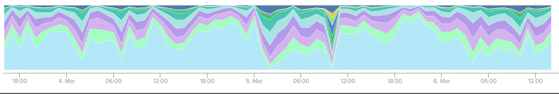
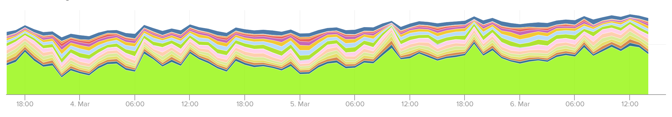
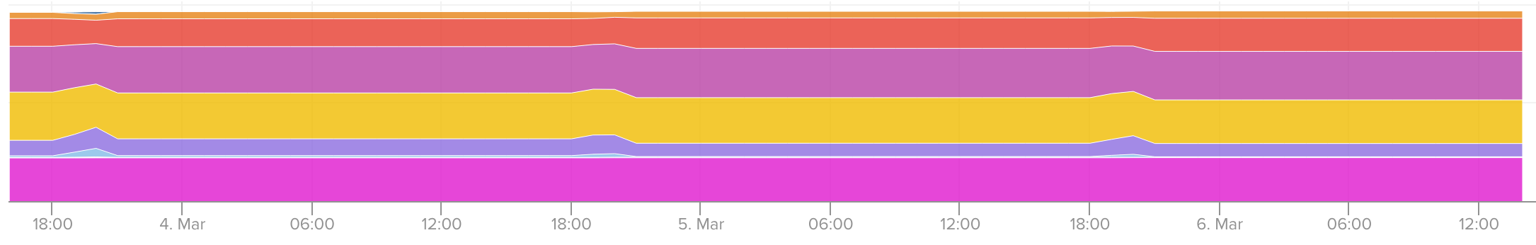
We’ve found that you can chart the clustering histogram and it produces some useful and aesthetically pleasing charts. What we look for in these charts is that we are maintaining the stratification of the buckets at our equilibrium point over time. Here are a couple of examples of charts from our monitoring software:
ABR: Always Be Re-clustering
When loading new data make sure you are re-clustering the table after each load. If you are trickle loading, you can separate the load and re-cluster process by re-clustering every several minutes rather than with each load. Since Snowflake supports concurrent DML, this is a good approach for maintaining low latency ingest times. The re-cluster command takes in a re-cluster "budget" argument named max_size which is the number of bytes that the compute warehouse will shuffle into optimal micro-partitions -- too little and your table degrades in its clustering status with each load. If you choose a number that is too high, Snowflake is smart enough to not waste compute cycles re-clustering beyond what is necessary. However, Snowflake may still re-cluster the table “too well”, meaning that it would be clustered beyond the point of diminishing returns for query performance per the Pareto principle.
As you load data and re-cluster, monitor the histogram and your re-cluster max_size amount. Keep loading data and tweaking the re-cluster amount until you have found an equilibrium point where each load plus re-cluster keeps the histogram steady in the desired state. Track the histogram over time, things may change and suddenly you may find that you were in the 00032 bucket on the high end and now you're in the 01024 bucket which would be bad. If this happens, tweak your re-cluster amount up to course correct.
Keep loading data and tweaking the re-cluster amount until you have found an equilibrium point where each load plus re-cluster keeps the histogram steady in the desired state.
In closing
Snowflake is a powerful database, but as a user you are still responsible for making sure that the data is laid out optimally to maximize query performance. If you follow the steps outlined in this post, you will remove a bunch of factors that could lead to less than optimal query performance. Here is a summary of the steps:
- When building a new clustered table in Snowflake, choose the cluster keys based on expected query workload.
- Load data and then manually re-cluster the table over and over again until cluster histogram reaches equilibrium.
- Fire up your regular ingestion process with periodic re-clustering. Inspect the clustering histogram and tweak the re-cluster amount until you find an equilibrium point that keeps the clustering from degrading.
- Monitor the histogram over time to ensure that you are not degrading into higher buckets slowly or if there is an unexpected change in your data composition.
Acknowledgements
Ashton Hepburn for his tireless work on our data loader and re-clustering infrastructure at Localytics. Thierry Cruanes and Benoit Dageville and the rest of the Snowflake team for guiding us through optimizing our environment.
Photo Credit: James Padolsey via Unsplash